Follow along
You can download this .Rmd file below if you’d like to follow along. I do have a few hidden notes you can disregard. This document is a distill_article, so you may want to change to an html_document to knit. You will also need to delete any image references to properly knit, since you won’t have those images.
Resources
- h2o in R cheatsheet
- h20.ai online documentation
- h20.ai booklet
- noRth talk on using autoML in R by Erin LeDell, Chief Machine Learning Scientist at
H20.ai. If you search the internet for Erin LeDell, you will find many more videos on this and similar topics.
Set up
First, we load the libraries we will use. There will be some new ones you’ll need to install. You also need to have Java installed - do that here first, before installing the h2o library. The version needs to be version 8, 9, 10, 11, 12, or 13, and I was required to create an oracle account. You can check to see if you already have java installed by typing java -version into the terminal. If you do this inside of R, make sure you are in your base directory - you can use the command cd .. to move up in your folder structure. After Java is installed, then install h2o.
library(tidyverse)         # for reading in data, graphing, and cleaning
library(tidymodels)        # for modeling ... tidily
library(lubridate)         # for dates
library(moderndive)        # for King County housing data
library(patchwork)         # for combining plots nicely
library(rmarkdown)         # for paged tables
library(h2o)               # use R functions to access the H2O machine learning platform
theme_set(theme_minimal()) # my favorite ggplot2 theme :)
Then we load the data we will use throughout this tutorial and do some modifications. As I mentioned before, I wouldn’t need to take the log here, but I do so I can compare to other models, if desired.
Introduction
Initiate our H2O instance. This should work without error as long as you have installed one of the Java versions indicated above.
h2o.init()
Connection successful!
R is connected to the H2O cluster:
H2O cluster uptime: 1 days 3 hours
H2O cluster timezone: America/Chicago
H2O data parsing timezone: UTC
H2O cluster version: 3.32.0.1
H2O cluster version age: 6 months and 5 days !!!
H2O cluster name: H2O_started_from_R_llendway_cgp501
H2O cluster total nodes: 1
H2O cluster total memory: 2.48 GB
H2O cluster total cores: 4
H2O cluster allowed cores: 4
H2O cluster healthy: TRUE
H2O Connection ip: localhost
H2O Connection port: 54321
H2O Connection proxy: NA
H2O Internal Security: FALSE
H2O API Extensions: Amazon S3, XGBoost, Algos, AutoML, Core V3, TargetEncoder, Core V4
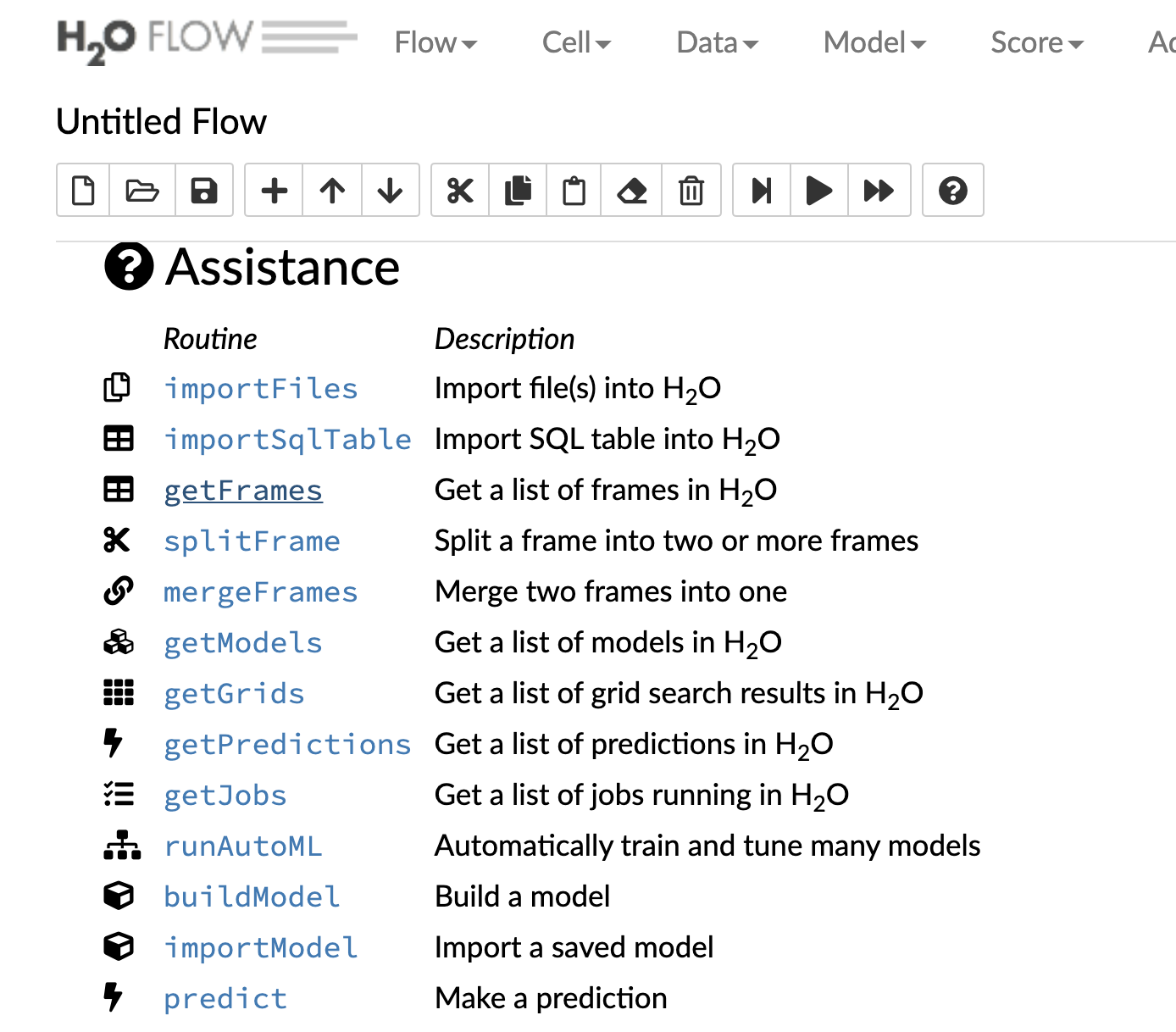
R Version: R version 4.0.2 (2020-06-22) You can also go to http://localhost:54321/flow/index.html in a web browser to see the flow. Think of it as us using R to interface with that webpage.
First, let’s read data into H2O. The destination_frame argument allows us to name the dataset in H2O.
house_h2o <- as.h2o(house_prices,
                    destination_frame = "house_prices")
  |
  |                                                            |   0%
  |
  |============================================================| 100%
Next, split the data into training and testing. Again, we can name the datasets we create in H2O using the destination_frames argument.
house_splits <- h2o.splitFrame(
  data = house_h2o,
  ratios = c(.75), #prop to training
  seed = 494,
  destination_frames = c("house_train", "house_test"))

house_train <- house_splits[[1]]
house_test <- house_splits[[2]]
We can list what we have in H2O using h2o.ls(). It will have all three I named and maybe more (I’m not exactly sure why).
h2o.ls()
And now that I have those data frames in H2O, I could actually do some inspection of them there (this link will only work if you are actually coding along since you will need to have the data loaded there). For example, I can click on getFrames and it will give a preview of what is currently in H2O, like in the image below on the right.
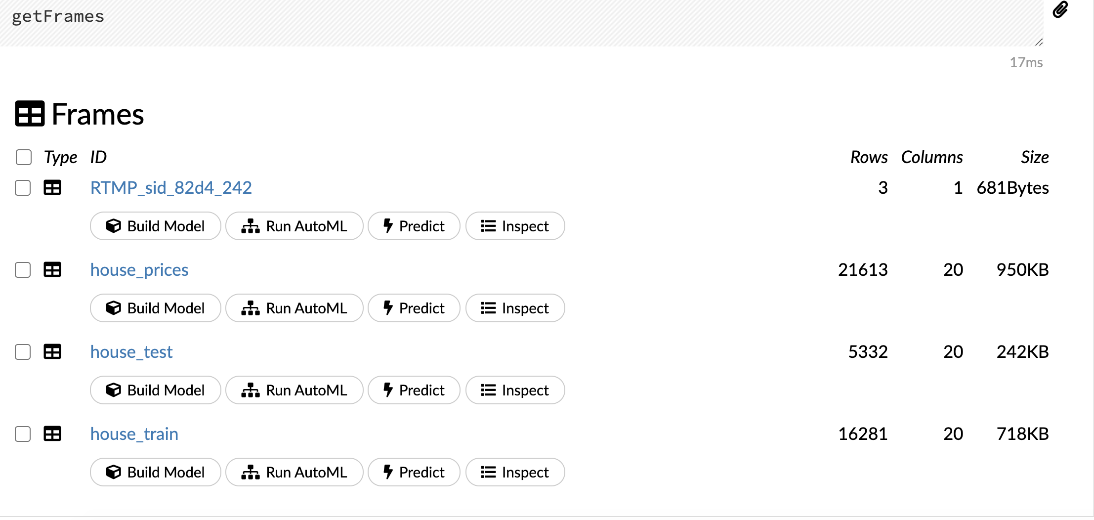
I could even do the modeling there, using the buildModel function! I’m not going to do that now, but I encourage you to play around with it. You should find that it’s very similar to the functions we will work with in R.
Now, let’s explore some of the models we could use, starting with a random forest. Similar to tidymodels or any other modeling framework you might use, there are a lot of options. I won’t cover all of them, but you can check them out by searching for h2o.randomForest in the help.
In this example, I will do the following:
- Define the outcome variable, y, as
log_price. I chose not to define the predictor variables, which means it will use everything except the outcome as predictors.
- Define the training data.
- Name the model with
model_idargument.
- Define the number of folds for k-fold cross-validation.
- Set a seed for reproducibility.
- Define the maximum run time in seconds.
rf_mod <- h2o.randomForest(y = "log_price",
                           training_frame = house_train,
                           model_id = "rand_for",
                           nfolds = 5,
                           seed = 494,
                           max_runtime_secs = 180)
  |
  |                                                            |   0%
  |
  |=                                                           |   1%
  |
  |==                                                          |   4%
  |
  |=====                                                       |   8%
  |
  |=======                                                     |  11%
  |
  |=========                                                   |  15%
  |
  |============                                                |  19%
  |
  |==============                                              |  23%
  |
  |================                                            |  27%
  |
  |==================                                          |  31%
  |
  |====================                                        |  34%
  |
  |=======================                                     |  38%
  |
  |=========================                                   |  42%
  |
  |===========================                                 |  45%
  |
  |=============================                               |  48%
  |
  |===============================                             |  51%
  |
  |=================================                           |  55%
  |
  |===================================                         |  58%
  |
  |====================================                        |  61%
  |
  |=======================================                     |  65%
  |
  |=========================================                   |  68%
  |
  |==========================================                  |  71%
  |
  |============================================                |  73%
  |
  |=============================================               |  75%
  |
  |===============================================             |  78%
  |
  |================================================            |  80%
  |
  |==================================================          |  83%
  |
  |===================================================         |  84%
  |
  |====================================================        |  87%
  |
  |======================================================      |  90%
  |
  |=======================================================     |  92%
  |
  |=========================================================   |  95%
  |
  |=========================================================== |  98%
  |
  |============================================================| 100%
And we can look at summaries of the model fit. You may be wondering why the evaluation metrics shown in the first set of output, labeled “H2ORegressionMetrics” are different from those in the mean column of the last data frame. I believe it is because in the first set of output, the predictions are combined to compute the metrics whereas in the dataframe, a metric is computed for each fold and then averaged. That is what is stated here in the “How Cross-Validation is Calculated” section. To quote from that documentation:
For the main model, this is how the cross-validation metrics are computed: The 5 holdout predictions are combined into one prediction for the full training dataset (i.e., predictions for every row of the training data, but the model making the prediction for a particular row has not seen that row during training). This “holdout prediction” is then scored against the true labels, and the overall cross-validation metrics are computed.
print(rf_mod)
Model Details:
==============

H2ORegressionModel: drf
Model ID:  rand_for
Model Summary:
  number_of_trees number_of_internal_trees model_size_in_bytes
1              50                       50             5546267
  min_depth max_depth mean_depth min_leaves max_leaves mean_leaves
1        20        20   20.00000       7973       8842  8368.54000


H2ORegressionMetrics: drf
** Reported on training data. **
** Metrics reported on Out-Of-Bag training samples **

MSE:  0.005793527
RMSE:  0.07611522
MAE:  0.05406491
RMSLE:  0.01145995
Mean Residual Deviance :  0.005793527


H2ORegressionMetrics: drf
** Reported on cross-validation data. **
** 5-fold cross-validation on training data (Metrics computed for combined holdout predictions) **

MSE:  0.00560481
RMSE:  0.07486528
MAE:  0.05314042
RMSLE:  0.01127549
Mean Residual Deviance :  0.00560481


Cross-Validation Metrics Summary:
                               mean           sd  cv_1_valid
mae                     0.053143732 0.0015694906  0.05443047
mean_residual_deviance 0.0056056944  4.955201E-4 0.006207818
mse                    0.0056056944  4.955201E-4 0.006207818
r2                        0.8933201  0.008670776  0.87858534
residual_deviance      0.0056056944  4.955201E-4 0.006207818
rmse                     0.07481251  0.003313405  0.07878971
rmsle                   0.011267388  4.985276E-4 0.011881535
                        cv_2_valid  cv_3_valid   cv_4_valid
mae                    0.050745845 0.052516554  0.054534145
mean_residual_deviance 0.005003212 0.005248708 0.0059651094
mse                    0.005003212 0.005248708 0.0059651094
r2                      0.90137523  0.89714557   0.89464027
residual_deviance      0.005003212 0.005248708 0.0059651094
rmse                    0.07073338  0.07244797   0.07723412
rmsle                  0.010666678 0.010915209  0.011630003
                         cv_5_valid
mae                     0.053491656
mean_residual_deviance 0.0056036245
mse                    0.0056036245
r2                         0.894854
residual_deviance      0.0056036245
rmse                     0.07485736
rmsle                   0.011243518
We can extract just the first part, like this:
h2o.performance(rf_mod,
                xval = TRUE)
H2ORegressionMetrics: drf
** Reported on cross-validation data. **
** 5-fold cross-validation on training data (Metrics computed for combined holdout predictions) **

MSE:  0.00560481
RMSE:  0.07486528
MAE:  0.05314042
RMSLE:  0.01127549
Mean Residual Deviance :  0.00560481
We can also create a graph of variable importance.
h2o.varimp_plot(rf_mod)

We could also evaluate how well the model performs on the test data.
h2o.performance(model = rf_mod,
                newdata = house_test)
H2ORegressionMetrics: drf

MSE:  0.005737752
RMSE:  0.07574795
MAE:  0.05298699
RMSLE:  0.01141956
Mean Residual Deviance :  0.005737752
We can use the model to predict the outcome on new data.
pred_test <- h2o.predict(rf_mod,
                         newdata = house_test)
  |
  |                                                            |   0%
  |
  |============================================================| 100%
# make it an R data.frame
as.data.frame(pred_test)
We can also save the model. The force = TRUE will overwrite the model if it’s already there.
h2o.saveModel(rf_mod,
              path = "/Users/llendway/GoogleDriveMacalester/2020FALL/Advanced_DS/ads_website/_posts/2021-04-13-h2o",
              force = TRUE)
[1] "/Users/llendway/GoogleDriveMacalester/2020FALL/Advanced_DS/ads_website/_posts/2021-04-13-h2o/rand_for"And read it back in to use it later. Notice it’s named “rand_for”, which was the model_id I gave it back when we fit the model.
test <- h2o.loadModel(path = "/Users/llendway/GoogleDriveMacalester/2020FALL/Advanced_DS/ads_website/_posts/2021-04-13-h2o/rand_for")

# use the new model to predict on new data
prediction_test <- h2o.predict(test,
                         newdata = house_test)
  |
  |                                                            |   0%
  |
  |============================================================| 100%
# make it an R data.frame
as.data.frame(prediction_test)
A slighlty more complex example with tuning
In the previous model, we just used all of the default values for the tuning parameters. This time, we will tune the mtries parameter, which is the number of randomly sampled variables that are candidates at each split. We use the h2o.grid() function when we want to tune. If you wanted to tune more parameters, you would add them to the rf_params list.
rf_params <- list(mtries = c(3, 5, 7, 10))

rf_mod_tune <- h2o.grid(
  "randomForest",
  y = "log_price",
  training_frame = house_train,
  grid_id = "rand_for_tune",
  nfolds = 5,
  seed = 494,
  max_runtime_secs = 180,
  hyper_params = rf_params
  )
  |
  |                                                            |   0%
  |
  |============================================================| 100%
Next, we sort the results by rmse.
rf_perf <- h2o.getGrid(
  grid_id = "rand_for_tune",
  sort_by = "rmse"
)

print(rf_perf)
H2O Grid Details
================

Grid ID: rand_for_tune
Used hyper parameters:
  -  mtries
Number of models: 4
Number of failed models: 0

Hyper-Parameter Search Summary: ordered by increasing rmse
  mtries             model_ids                rmse
1      5 rand_for_tune_model_2 0.07488179092166132
2      7 rand_for_tune_model_3  0.0749112023899115
3     10 rand_for_tune_model_4 0.07526110515830671
4      3 rand_for_tune_model_1 0.07579556971578551
We use h2o.getModel() to choose the first model in the list from above, which will be the best model - the one with the smallest rmse.
best_rf <- h2o.getModel(rf_perf@model_ids[[1]])
Then, we evaluate the best model on the test data. Just like in the previous example, we could also save this model and use it later. I will skip that step here.
h2o.performance(model = best_rf,
                newdata = house_test)
H2ORegressionMetrics: drf

MSE:  0.005688724
RMSE:  0.07542363
MAE:  0.05301439
RMSLE:  0.01136836
Mean Residual Deviance :  0.005688724
Auto ML
H2O offers many different machine learning algorithms to use, including boosting (gradient boosting and XGBOOST), stacked ensembles, and deep learning. There is also an auto ML algorithm, which tries many different algorithms and puts the results on a leaderboard. There are many arguments you can change. In this example, I will use most of the defaults. You can read more details here. Let’s try it out!
aml <- h2o.automl(
  y = "log_price",
  training_frame = house_train,
  nfolds = 5,
  seed = 494,
  max_runtime_secs_per_model = 120,
  max_models = 10
)
  |
  |                                                            |   0%
  |
  |=                                                           |   2%
  |
  |==                                                          |   3%
  |
  |===                                                         |   5%
  |
  |====                                                        |   7%
  |
  |=====                                                       |   8%
  |
  |======                                                      |  11%
  |
  |=======                                                     |  11%
  |
  |=======                                                     |  12%
  |
  |========                                                    |  13%
  |
  |========                                                    |  14%
  |
  |=========                                                   |  15%
  |
  |=========                                                   |  16%
  |
  |==========                                                  |  16%
  |
  |==========                                                  |  17%
  |
  |===========                                                 |  18%
  |
  |===========                                                 |  19%
  |
  |============                                                |  19%
  |
  |============                                                |  21%
  |
  |=============                                               |  21%
  |
  |=============                                               |  22%
  |
  |==============                                              |  24%
  |
  |===============                                             |  24%
  |
  |===============                                             |  25%
  |
  |===============                                             |  26%
  |
  |================                                            |  26%
  |
  |================                                            |  27%
  |
  |============================================================| 100%
We can take a look at the leaderboard - change n to see more or fewer models.
print(aml@leaderboard,
      n = 10)
                           model_id mean_residual_deviance       rmse
1      GBM_1_AutoML_20210414_145747            0.004946030 0.07032802
2      GBM_5_AutoML_20210414_145747            0.004979559 0.07056599
3      GBM_2_AutoML_20210414_145747            0.004980562 0.07057310
4      GBM_3_AutoML_20210414_145747            0.005050799 0.07106898
5      GBM_4_AutoML_20210414_145747            0.005103994 0.07144224
6  XGBoost_3_AutoML_20210414_145747            0.005311748 0.07288174
7      DRF_1_AutoML_20210414_145747            0.005565699 0.07460361
8  XGBoost_1_AutoML_20210414_145747            0.005849319 0.07648084
9  XGBoost_2_AutoML_20210414_145747            0.006070725 0.07791486
10     GLM_1_AutoML_20210414_145747            0.006265746 0.07915647
           mse        mae      rmsle
1  0.004946030 0.05013409 0.01061924
2  0.004979559 0.05007461 0.01064223
3  0.004980562 0.05018989 0.01065484
4  0.005050799 0.05047216 0.01072535
5  0.005103994 0.05045897 0.01078796
6  0.005311748 0.05243210 0.01099025
7  0.005565699 0.05296334 0.01123630
8  0.005849319 0.05488541 0.01153573
9  0.006070725 0.05639028 0.01175664
10 0.006265746 0.05811367 0.01192215

[12 rows x 6 columns]
We can extract the best model (first in the leaderboard list).
best_mod <- as.vector(aml@leaderboard$model_id)[1]
best_mod
[1] "GBM_1_AutoML_20210414_145747"And see the details of the best model. We could save this model to use later, as we did with the first random forest model we created. I will skip that step.
best_auto <- h2o.getModel(best_mod)
best_auto
Model Details:
==============
H2ORegressionModel: gbm
Model ID: GBM_1_AutoML_20210414_145747
Model Summary:
number_of_trees number_of_internal_trees model_size_in_bytes
1 110 110 100025
min_depth max_depth mean_depth min_leaves max_leaves mean_leaves
1 6 6 6.00000 35 64 58.17273
H2ORegressionMetrics: gbm
** Reported on training data. **
MSE: 0.002846518
RMSE: 0.05335277
MAE: 0.03957865
RMSLE: 0.008077859
Mean Residual Deviance : 0.002846518
H2ORegressionMetrics: gbm
** Reported on cross-validation data. **
** 5-fold cross-validation on training data (Metrics computed for combined holdout predictions) **
MSE: 0.00494603
RMSE: 0.07032802
MAE: 0.05013409
RMSLE: 0.01061924
Mean Residual Deviance : 0.00494603
Cross-Validation Metrics Summary:
mean sd cv_1_valid
mae 0.0501341 7.29446E-4 0.050049435
mean_residual_deviance 0.0049460186 1.5085173E-4 0.005135245
mse 0.0049460186 1.5085173E-4 0.005135245
r2 0.90579545 0.0045276335 0.898309
residual_deviance 0.0049460186 1.5085173E-4 0.005135245
rmse 0.070321426 0.0010698918 0.07166062
rmsle 0.010617994 1.810597E-4 0.010842165
cv_2_valid cv_3_valid cv_4_valid
mae 0.04967257 0.05029413 0.051277976
mean_residual_deviance 0.004812066 0.0048809047 0.005079365
mse 0.004812066 0.0048809047 0.005079365
r2 0.90758127 0.9052192 0.90776557
residual_deviance 0.004812066 0.0048809047 0.005079365
rmse 0.069369055 0.06986347 0.07126966
rmsle 0.01046122 0.010539268 0.010781831
cv_5_valid
mae 0.049376387
mean_residual_deviance 0.0048225117
mse 0.0048225117
r2 0.91010225
residual_deviance 0.0048225117
rmse 0.069444306
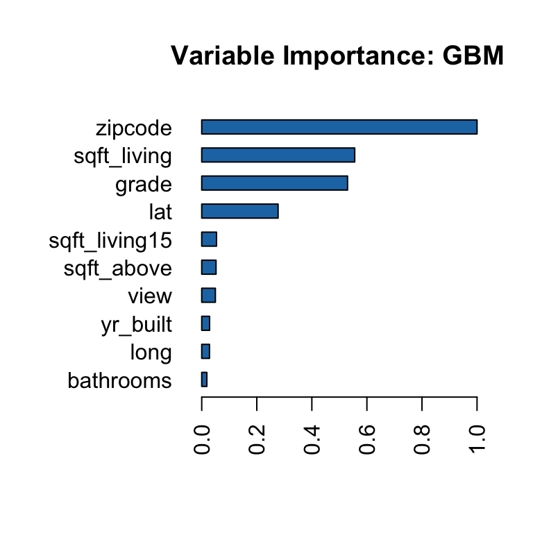
rmsle 0.010465484And we can do all the same things we did with other models we fit. Like creating a variable importance plot:
h2o.varimp_plot(best_auto)
Using it to predict the outcome with new data:
auto_pred <- h2o.predict(best_auto,
                         newdata = house_test)
  |
  |                                                            |   0%
  |
|============================================================| 100%as.data.frame(auto_pred)
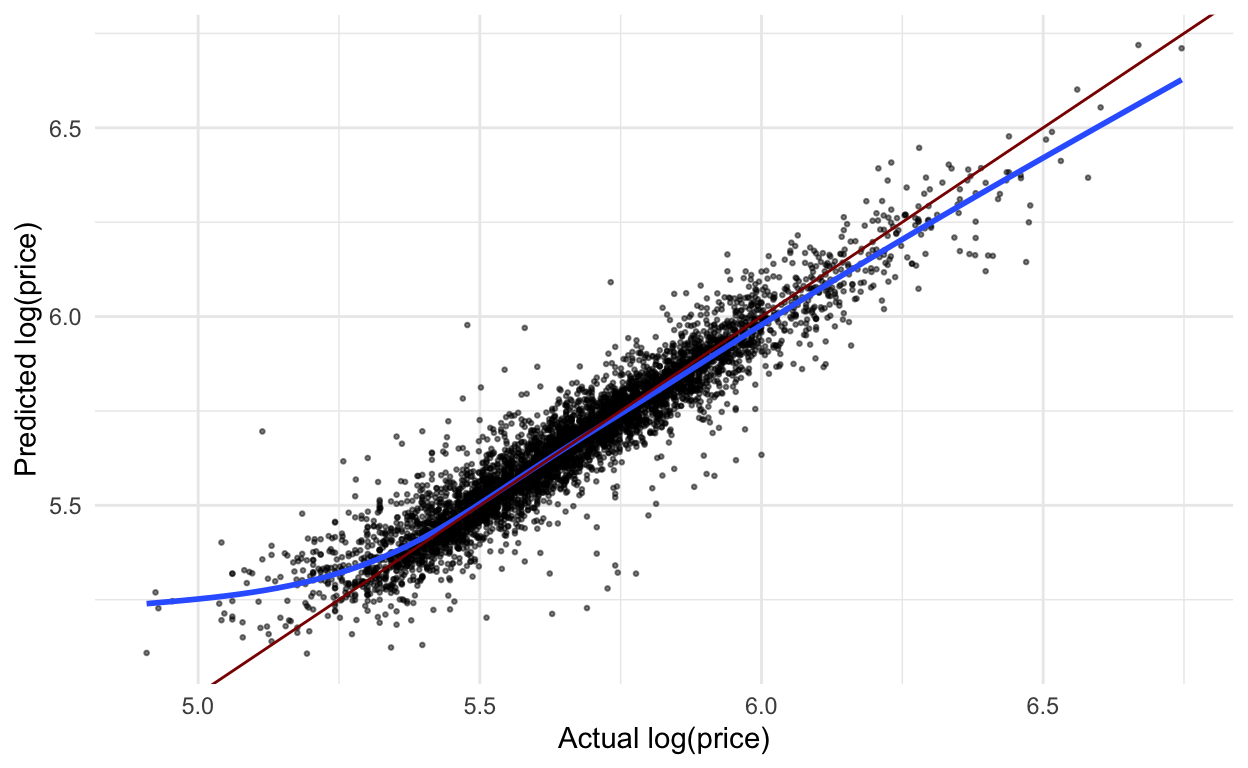
And creating a nice plot of predicted vs. actual values:
predictions <- as.data.frame(house_test) %>%
  bind_cols(as.data.frame(auto_pred))

predictions  %>%
  ggplot(aes(x = log_price,
             y = predict)) +
  geom_point(alpha = .5,
             size = .5) +
  geom_smooth(se = FALSE) +
  geom_abline(slope = 1,
              intercept = 0,
              color = "darkred") +
  labs(x = "Actual log(price)",
       y = "Predicted log(price)")
Explore!
There is so much more that you can do with this package than I have shown you. I encourage you to explore the resources I linked to above and try it out!