Follow along
You can download this .Rmd file below if you’d like to follow along. I do have a few hidden notes you can disregard. This document is a distill_article, so you may want to change to an html_document to knit. You will also need to delete any image references to properly knit, since you won’t have those images.
Resources
- stacks R package documentation by Simon Couch and Max Kuhn and Simon’s lightnight talk. I highly recommend watching the lightning talk first for a quick, entertaining overview.
- Hands on Machine Learning chapter on stacking by Bradley Boehmke & Brandon Greenwell. This does not discuss the
stackspackage but gives a good overview of the stacking process.
Set up
Here, we load libraries we will use and load the King County house price data.
library(tidyverse)         # for reading in data, graphing, and cleaning
library(tidymodels)        # for modeling ... tidily
library(stacks)            # for stacking models
library(glmnet)            # for regularized regression, including LASSO
library(ranger)            # for random forest model
library(kknn)              # for knn model
library(naniar)            # for examining missing values (NAs)
library(lubridate)         # for date manipulation
library(moderndive)        # for King County housing data
library(vip)               # for variable importance plots
library(rmarkdown)         # for paged tables
theme_set(theme_minimal()) # my favorite ggplot2 theme :)
data("house_prices")

house_prices %>%
  slice(1:5)
This isn’t so new
The general idea of stacking is to combine predictions from many different models (called candidate models, candidate ensemble members, base learners, and probably other names I don’t know yet) into one “super” predictor. For example, we could fit a regression model, a decision tree, and a KNN model to the King County house price data and then average the predicted values from each of those models for a final prediction. That’s a simplified version of what we’ll do, but if you understand that, you’ll understand stacking. We will use the stacks package to help us out. I think it has one of the greatest hex stickers!

We have seen something similar to this before: bagging and random forest models. Let’s do a little review and remember what a random forest model is:
- Take a bootstrap sample of the data (sample of the same size as the original sample, with replacement).
- Build a modified decision tree. At each split, only consider a random sample of the \(p\) predictors, \(m\). A common choice in regression models is \(m = \frac{p}{3}\) and in classification models is \(m = \sqrt{p}\) (\(m\) can also be treated as a tuning parameter). This will limit how often a dominant predictor can be used and will make the trees less correlated.
- Repeat steps 1 and 2 many times (at least 50). Call the number of trees B.
- New observations will have a predicted value of the average predicted value from the B trees (or could also be the most common category for classification).
Bagging is a form of random forest with \(m=p\).
To review, let’s use our new tidymodels functions to fit a random forest model to the King County house price data.
Because I am going to use this later as one of the stacking models and some of those models will predict log(price), I am also going to predict log(price) in this model, even though I wouldn’t have to.
set.seed(327) #for reproducibility

house_prices <- house_prices %>%
  mutate(log_price = log(price, base = 10)) %>%
  select(-price)

# Randomly assigns 75% of the data to training.
house_split <- initial_split(house_prices,
                             prop = .75)
house_split
<Analysis/Assess/Total>
<16209/5404/21613>
#<training/testing/total>
house_training <- training(house_split)
house_testing <- testing(house_split)
First, create the recipe. With decision trees (and therefore random forests), we don’t have to do as much prepping of the data.
ranger_recipe <-
  recipe(formula = log_price ~ .,
         data = house_training) %>%
  step_date(date,
            features = "month") %>%
  # Make these evaluative variables, not included in modeling
  update_role(all_of(c("id",
                       "date")),
              new_role = "evaluative")
Now, define the model. We could tune the mtry (this is \(m\), the number of randomly sampled predictors considered at each split), min_n, and trees parameters, but to simplify, we’ll just set them to specific values.
We’ll use mtry = 6, which is about 1/3 of the number of predictor variables, a commonly chosen value of mtry; min_n = 10 (the minimum number of data points in a node that are required for the node to be split further, ie. anything smaller and it won’t be split more); and trees = 200, which is the number of decision trees that will be used in the ensemble.
ranger_spec <-
  rand_forest(mtry = 6,
              min_n = 10,
              trees = 200) %>%
  set_mode("regression") %>%
  set_engine("ranger")
Next, we create the workflow:
ranger_workflow <-
  workflow() %>%
  add_recipe(ranger_recipe) %>%
  add_model(ranger_spec)
And then we fit the model (be sure to have the ranger library installed first, although it doesn’t need to be loaded):
ranger_fit <- ranger_workflow %>%
  fit(house_training)

ranger_fit
══ Workflow [trained] ════════════════════════════════════════════════
Preprocessor: Recipe
Model: rand_forest()

── Preprocessor ──────────────────────────────────────────────────────
1 Recipe Step

• step_date()

── Model ─────────────────────────────────────────────────────────────
Ranger result

Call:
 ranger::ranger(x = maybe_data_frame(x), y = y, mtry = min_cols(~6,      x), num.trees = ~200, min.node.size = min_rows(~10, x), num.threads = 1,      verbose = FALSE, seed = sample.int(10^5, 1))

Type:                             Regression
Number of trees:                  200
Sample size:                      16209
Number of independent variables:  19
Mtry:                             6
Target node size:                 10
Variable importance mode:         none
Splitrule:                        variance
OOB prediction error (MSE):       0.005843126
R squared (OOB):                  0.8877044
With random forests, we can estimate the prediction error using the “out-of-bag” error (OOB error). Remember, with bootstrap samples, we sample with replacement so some observations are in the sample multiple times while others aren’t in it at all. The OOB observations are those that are not in the bootstrap sample. Find predicted values for OOB observations by averaging their predicted value for the trees where they were OOB. The OOB MSE is part of the fit() output and we can take the square root to get the RMSE.
# OOB error (MSE) ... yeah, it took me a while to find that.
ranger_fit$fit$fit$fit$prediction.error
[1] 0.005843126#OOB RMSE
sqrt(ranger_fit$fit$fit$fit$prediction.error)
[1] 0.07644034We will also evaluate this using cross-validation because we’ll need that later when we stack models. I’m using the same seed I used in the previous tutorial when we fit a linear regression because I want the same folds.
We also define a couple things that will be used in stacking. The metric_set() tells it we are using RMSE. We also use the control_stack_resamples() function to assure the assessment set predictions and and workflow used to fit the resamples is stored.
set.seed(1211) # for reproducibility
house_cv <- vfold_cv(house_training, v = 5)

metric <- metric_set(rmse)
ctrl_res <- control_stack_resamples()

ranger_cv <- ranger_workflow %>%
  fit_resamples(house_cv,
                metrics = metric,
                control = ctrl_res)

# Evaluation metrics averaged over all folds:
collect_metrics(ranger_cv)
Notice that the cross-validated RMSE is about the same as the OOB RMSE, but cross-validated version takes longer to run (it is fitting 200 X 5 decision trees!). This is also a lot smaller than the RMSE obtained from the regular linear regression model or the lasso model.
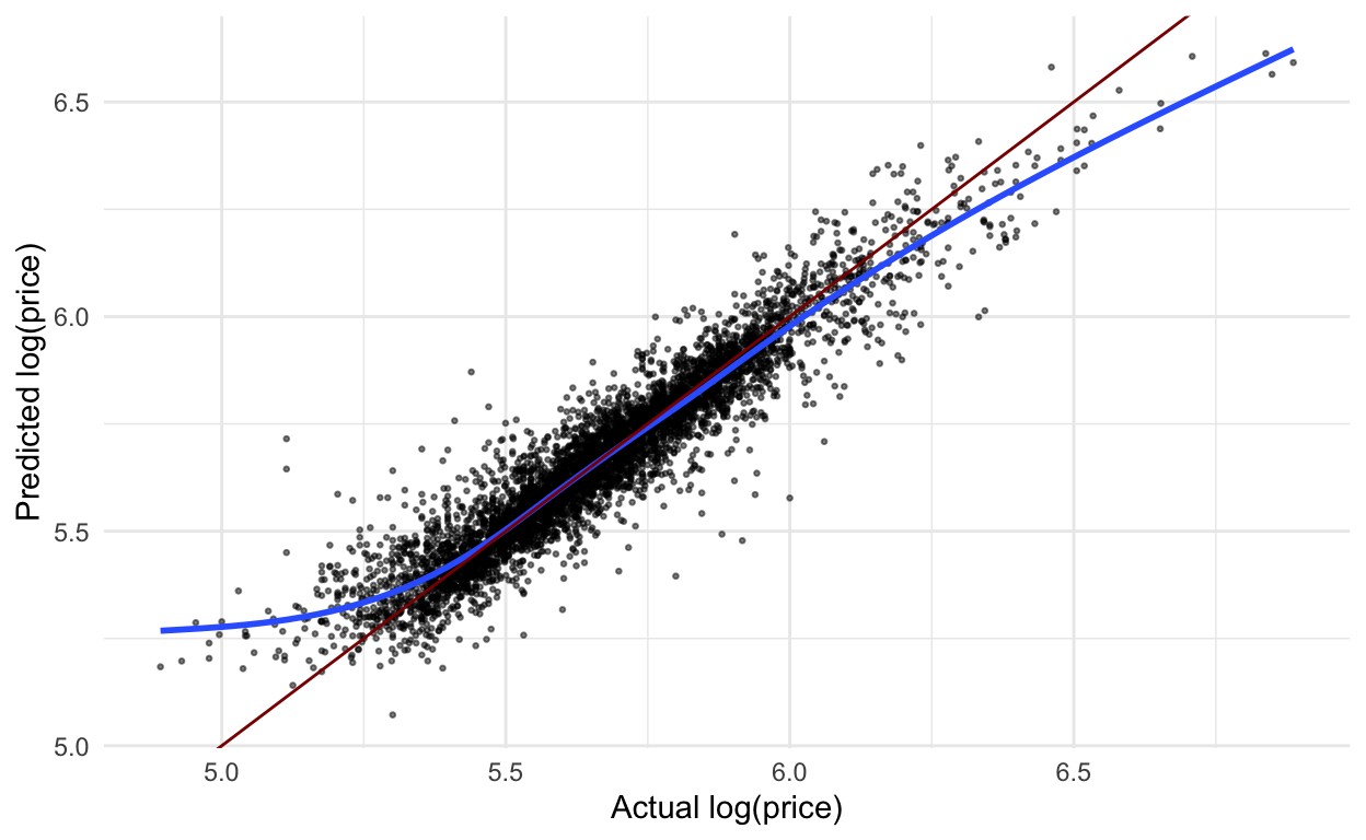
Just for fun, before stacking, let’s also apply this model to the test data and plot the predicted vs. actual log price. Compared to this same graph from the linear regression model, this looks much better! There are still some issues with really small and really large values, but not nearly as bad.
ranger_workflow %>%
  last_fit(house_split) %>%
  collect_predictions() %>%
  ggplot(aes(x = log_price,
             y = .pred)) +
  geom_point(alpha = .5,
             size = .5) +
  geom_smooth(se = FALSE) +
  geom_abline(slope = 1,
              intercept = 0,
              color = "darkred") +
  labs(x = "Actual log(price)",
       y = "Predicted log(price)")

Creating more candidate models
In order to create a stacked model, we first have to create the individual models. We have the random forest we just created, ranger_cv. Let’s also recreate the lasso model from the previous tutorial, but add a couple missing pieces. I do that below. We will end up with 10 models that will flow into the stacked model, since we tune 10 penalty parameters.
# lasso recipe and transformation steps
house_recipe <- recipe(log_price ~ .,
                       data = house_training) %>%
  step_rm(sqft_living15, sqft_lot15) %>%
  step_log(starts_with("sqft"),
           -sqft_basement,
           base = 10) %>%
  step_mutate(grade = as.character(grade),
              grade = fct_relevel(
                        case_when(
                          grade %in% "1":"6"   ~ "below_average",
                          grade %in% "10":"13" ~ "high",
                          TRUE ~ grade
                        ),
                        "below_average","7","8","9","high"),
              basement = as.numeric(sqft_basement == 0),
              renovated = as.numeric(yr_renovated == 0),
              view = as.numeric(view == 0),
              waterfront = as.numeric(waterfront),
              age_at_sale = year(date) - yr_built)%>%
  step_rm(sqft_basement,
          yr_renovated,
          yr_built) %>%
  step_date(date,
            features = "month") %>%
  update_role(all_of(c("id",
                       "date",
                       "zipcode",
                       "lat",
                       "long")),
              new_role = "evaluative") %>%
  step_dummy(all_nominal(),
             -all_outcomes(),
             -has_role(match = "evaluative")) %>%
  step_normalize(all_predictors(),
                 -all_nominal())

#define lasso model
house_lasso_mod <-
  linear_reg(mixture = 1) %>%
  set_engine("glmnet") %>%
  set_args(penalty = tune()) %>%
  set_mode("regression")

# create workflow
house_lasso_wf <-
  workflow() %>%
  add_recipe(house_recipe) %>%
  add_model(house_lasso_mod)

# penalty grid - changed to 10 levels
penalty_grid <- grid_regular(penalty(),
                             levels = 10)

# add ctrl_grid - assures predictions and workflows are saved
ctrl_grid <- control_stack_grid()

# tune the model using the same cv samples as random forest

house_lasso_tune <-
  house_lasso_wf %>%
  tune_grid(
    resamples = house_cv,
    grid = penalty_grid,
    metrics = metric,
    control = ctrl_grid
    )
We will create one more model type - K-nearest neighbors. We can use the same recipes and step as in the lasso model. So, we define the model, leaving the number of neighbors (k) to be tuned; create the workflow; and tune the model (install kknn package first - don’t need to load):
# create a model definition
knn_mod <-
  nearest_neighbor(
    neighbors = tune("k")
  ) %>%
  set_engine("kknn") %>%
  set_mode("regression")

# create the workflow
knn_wf <-
  workflow() %>%
  add_model(knn_mod) %>%
  add_recipe(house_recipe)

# tune it using 4 tuning parameters
knn_tune <-
  knn_wf %>%
  tune_grid(
    house_cv,
    metrics = metric,
    grid = 4,
    control = ctrl_grid
  )
Stacking
Now that we have our set of candidate models (1 random forest, 10 lasso, and 4 knn), we’re ready to stack! We’re going to follow the process laid out on the stacks webpage.
First, create the stack. Notice in the message, it has removed some of the candidate models, likely since they were too similar to other lasso models.
house_stack <-
  stacks() %>%
  add_candidates(ranger_cv) %>%
  add_candidates(house_lasso_tune) %>%
  add_candidates(knn_tune)
We can look at the predictions from the candidate models in a tibble. The first column is the actual outcome, log_price and the other columns are the predictions from the various models. They are given names that make sense - how nice! Note that with classification models, there will be a column for each model for each level of the outcome variable. So, for a binary response there would be two prediction columns for each model.
as_tibble(house_stack)
Now, as mentioned at the beginning, we want to blend the predictions from each model together to form an even better overall prediction. LASSO will be used to do this via the blend_predictions() function.
From the documentation, blend_predictions() “evaluates a data stack by fitting a regularized model on the assessment predictions from each candidate member to predict the true outcome. This process determines the ‘stacking coefficients’ of the model stack. The stacking coefficients are used to weight the predictions from each candidate (represented by a unique column in the data stack), and are given by the betas of a LASSO model fitting the true outcome with the predictions given in the remaining columns of the data stack.”
Doing this with our models, we see only two models have non-zero coefficients:
house_blend <-
  house_stack %>%
  blend_predictions()

house_blend
# A tibble: 3 × 3
  member        type             weight
  <chr>         <chr>             <dbl>
1 ranger_cv_1_1 rand_forest      1.02
2 knn_tune_1_4  nearest_neighbor 0.0173
3 knn_tune_1_3  nearest_neighbor 0.0138
We can see the rmse for the various penalty parameters:
house_blend$metrics %>%
  filter(.metric == "rmse")
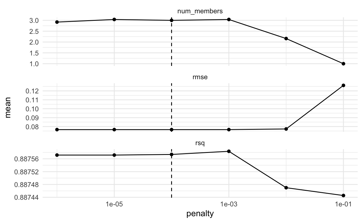
We can examine some plots to see if we need to adjust the penalty parameter at all. First, a set of three plots with penalty on the x axis. We seem to have captured the smallest RMSE so I won’t adjust the penalty at all. You can change the penalty as an argument in the blend_predictions() function.
autoplot(house_blend)
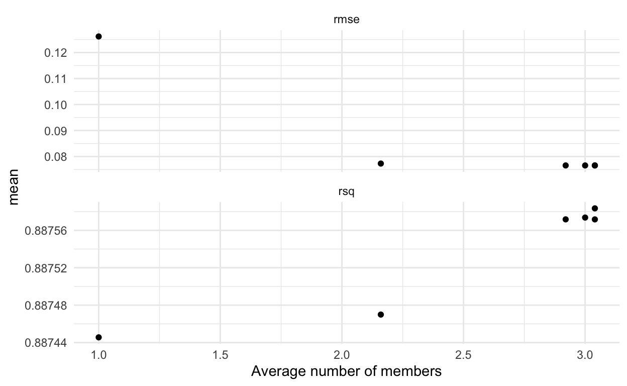
We can also examine the plot with average number of members on the x-axis. You might wonder where the average comes from - it is because we are using cross-validation. So, we get different results for each penalty depending on the fold being left out. (Thanks to Max Kuhn and Simon Couch’s quick response to my request to fix the axes of the plot - yay!).
autoplot(house_blend, type = "members")
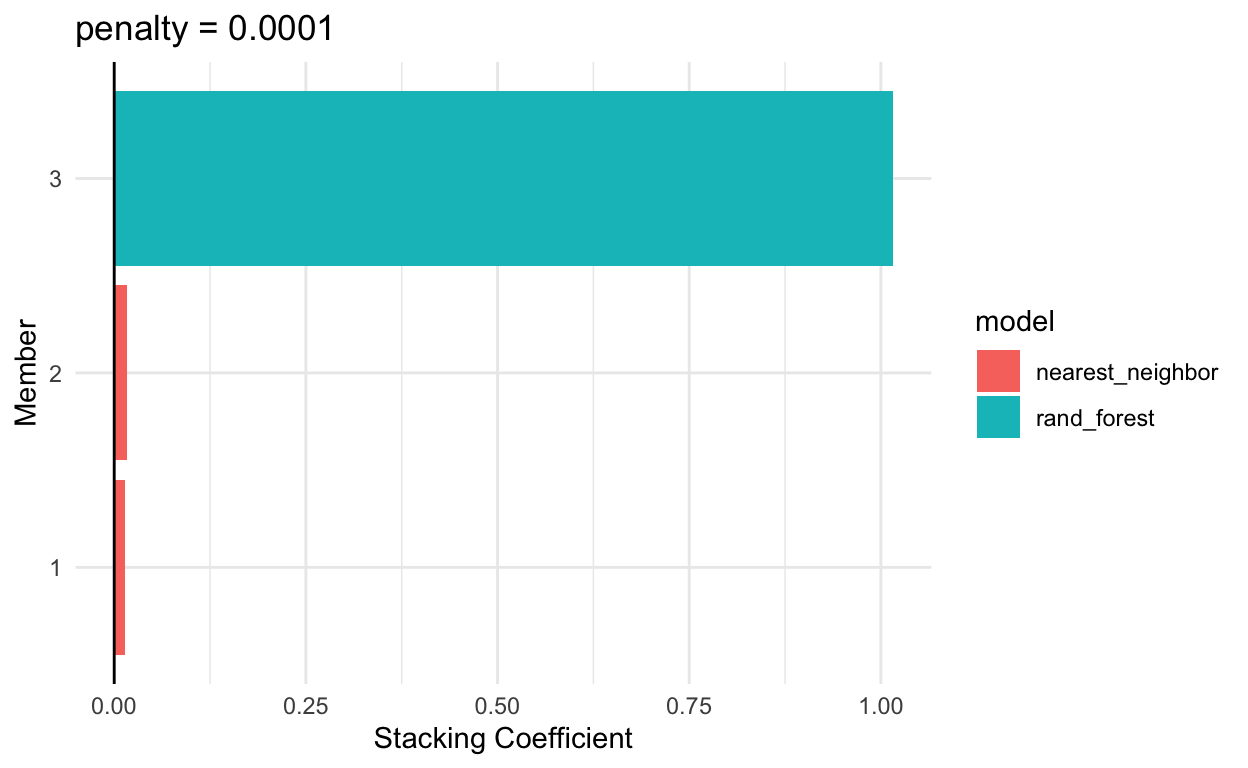
The last plot we might examine shows the blending weights for the top ensemble members.
autoplot(house_blend, type = "weights")
The last thing we need to do is fit the candidate models with non-zero stacking coefficients to the full training data. We use fit_members() to do that.
house_final_stack <- house_blend %>%
  fit_members()

house_final_stack
# A tibble: 3 × 3
  member        type             weight
  <chr>         <chr>             <dbl>
1 ranger_cv_1_1 rand_forest      1.02
2 knn_tune_1_4  nearest_neighbor 0.0173
3 knn_tune_1_3  nearest_neighbor 0.0138
Now we can use this just as we would use a single model. For example, we can predict with it on new data and create the same predicted vs. actual plot we made above.
house_final_stack %>%
  predict(new_data = house_testing) %>%
  bind_cols(house_testing) %>%
  ggplot(aes(x = log_price,
             y = .pred)) +
  geom_point(alpha = .5,
             size = .5) +
  geom_smooth(se = FALSE) +
  geom_abline(slope = 1,
              intercept = 0,
              color = "darkred") +
  labs(x = "Actual log(price)",
       y = "Predicted log(price)")